Internal Sorting
각각의 sorting algorithm을 비교하기 위해 # of comparison, # of swap을 기준으로 삼는다.
1. $\Theta(n^2)$ Sorting Algorithms
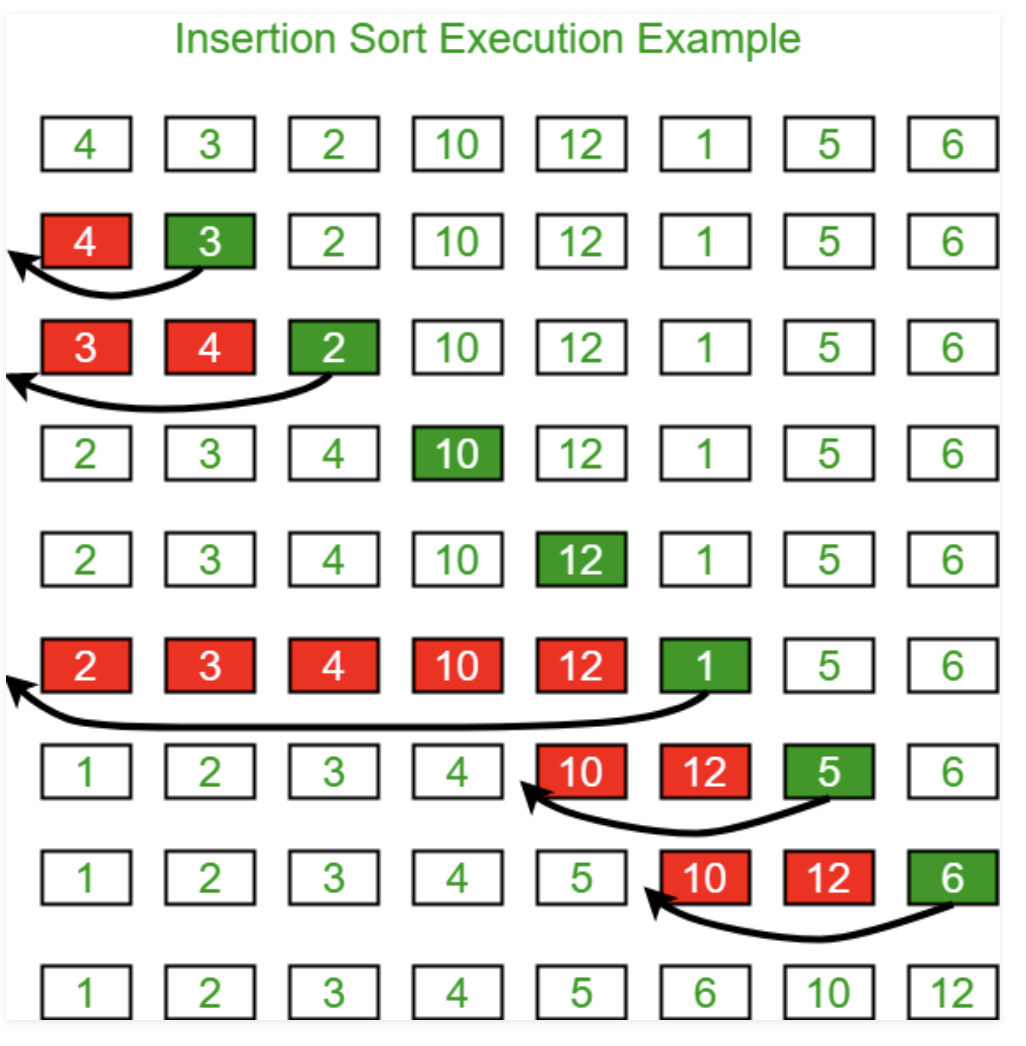
1-1. Insertion Sort
(1) 초기에 output은 비어있다.
(2) 각각의 item을 알맞은 장소에 삽입한다.
static <E extends Comparable<? super E>>
void InsertionSort(E[] A){

    for(int i = 1; i < A.length; i++){
    	for(int j = i; (j>0) && (A[j].compareTo(A[j-1])<0); j--){
        	DSutil.swap(A, j, j-1);
        }
    }
}
Best Case : 0 swaps, n - 1 comparisons
Worst Case : $n^2/2$ swaps and comparisons
Average Case : $n^2/4$ swaps and comparisons
Insertion sort는 거의 정렬되어있을 때 가장 효율적이다.
1-2. Bubble Sort
(1) 초기에 output은 비어있다.
(2) k번째 iteration마다 k번째 아이템이 array[k]에 위치한다.
(3) 끝에서부터 작은 item이 있을 때 swap한다.

static <E extends Comparable<? super E>>
void BubbleSort(E[] A){

    for(int i = 0; i < A.length-1; i++){
    	for(int j = A.length-1; j>i; j--){
        	if(A[j].compareTo(A[j-1]) < 0){
            	DSutil.swap(A, j, j-1);
            }
        }
    }
}
Best Case : 0 swaps, $n^2/2$ comparisons
Worst Case : $n^2/2$ swaps and comparisons
Average Case : $n^2/4$ swaps and $n^2/2$ comparisons
1-3. Selection Sort
기본적으로 bubble sort와 비슷하다.(n번째 iteration 때, n번째 item을 array[n]으로)
Selection sort는 n개의 item들을 scan한 이후 가장 작은 element와 맨 첫번째 element를 swap한다.

Best Case : 0 swaps (n-1 for bad swap), $n^2/2$ comparisons
Worst Case : n-1 swaps and $n^2/2$ comparisons
Average Case : O(n) swaps and $n^2/2$comparisons
Better than Bubble sort!(# of swap)
1-4. Summary

selection의 경우 swap을 잘 설계한다면 best case에서 0번 swap할 수 있다.
앞선 3가지의 sorting은 모두 근접한 item을 swap하는 방식으로 작동한다. 이러한 sorting 방식을 Exchange sorting이라 칭한다.
Exchange Sorting의 경우 average case에서 $\Omega(n^2)$의 시간복잡도를 가진다.
prove)
(1) n!의 permutation이 있다고 가정하자.
(2) 그 permutation을 X라고 하고(ex) 4-1-3-2), 역순을 X'라고 한다.(2-3-1-4)
(3) X와 X'의 exchange 횟수를 합하면 n(n-1)/2이다.
(4) 따라서 평균적으로 $\Omega(n^2)$의 시간복잡도를 가진다.
2. Shellsort
Main Idea : 두개의 sub array로 나누어서 recursive하게 sort
$x_e$ = index가 짝수인 원소들의 집합
$x_o$ = Index가 홀수인 원소들의 집합
이 둘이 정렬되어있다고 가정하고 insertion sort를 수행함.
(-> 거의 다 정렬되어 있기 때문에 효율적)


pass2 result : 14-10-27-19-35-33-42-44
pass3 result : 10-14-19-27-33-35-42-44
static <E extends Comparable<? super E>>
void ShellSort(E[] A){

    for(int i = A.length/2; i>=2; i/=2){
    	for(int j = 0; j < i; j++){
        	inssort2(A, j, i);
        }
        inssort2(A, 0, 1); //last insertion sort
    }
}

static <E extends Comparable<? super E>>
void inssort2(E[] A, int start, int incr){

    for(int i = start+incr; i<A.length; i+=incr){
    	for(int j = i; (j < i)&&(A[j].compareTo(A[j-incr])<0); j-=incr){
        	DSutil.swap(A, j, j-incr);
        }
    }
}
마지막에 insertion sort를 수행하기 때문에 무조건 정렬된다.
모든 insertion sort를 수행할 때 대부분 정렬이 되어있는 상태이기 때문에, 효율적으로 동작한다.
average case의 시간 복잡도는 O($n^{1.5}$)이다.
3. Merge Sort
Divide and Conquer : 재귀적으로 들어온 배열을 절반으로 나누어 각각 정렬을 수행한다.

static <E extends Comparable<? super E>>
void mergesort(E[] A, E[] temp, int l, int r){
    int mid = (l + r) / 2;
    if(l == r) return;
    mergesort(A, temp, l, mid);
    mergesort(A, temp, mid+1, r);
    for(int i = l; i <= r; i++) // copy subarray
    	temp[i] = A[i]
    //Do the merge operation back to A
    int i1 = l; int i2 = mid+1;
    for(int curr=l; curr <= r; curr++){
    	if(i1 == mid+1) // left subarray exhausted
        	A[curr] = temp[i2++];
        else if(i2 > r)
        	A[curr] = temp[i1++];
        else if(temp[i1].compareTo(temp[i2])<0)
        	A[curr] = temp[i1++];
        else A[curr] = temp[i2++];
    }
}
각각 왼쪽 절반과 오른쪽 절반에 index i1, i2를 두고 비교하며 A[]에 하나씩 넣는다.
이때 최적화 방법이 두가지가 존재하는데,
(1) i1, i2의 경계를 체크하는 것을 없애는 것과
(2) Threshold보다 작을 경우 insertion sort로 수행하는 것
void MergeSortImproved(E[] A, E[] temp, int l, int r){
    int i, j, k, mid = (l+r) / 2;
    if(l == r) return;
    if((mid - l) >= Threhold){
    	MergeSortImproved(A, temp, l, mid);
    }
    else inssort(A, l, mid-l+1);
    if((r-mid) > Threshold){
    	mergesort(A, temp, mid+1, r);
    }
    else inssort(A, temp, mid+1, r);
    //Do merge. First, copy 2 halves to temp.
    for(i = l; i <=mid; i++) temp[i] = A[i];
    for(j = 1; j <= r-mid; j++) temp[r-j+1] = A[j + mid];
    //Merge sublists back tp array
    for(i = l; j = r, k = l; k <= r; k++){
    	if(temp[i].compareTo(temp[j]) < 0)
        	A[k] = temp[i++];
        else A[k] = temp[j--];
    }
}
temp에 각각 절반의 정렬된 배열을 반대로 넣어줌으로써 경계값을 체크할 필요 없이 최적화했다.
best, average, worst case = $\Theta(n log n)$
Mergesort는 linked list를 sorting하는데 아주 좋다. -> Sequential access만 사용하기 때문
Mergesort는 두배의 space를 사용한다.
5. Quicksort
또다른 divide and conqure approach
input array가 주어질 때. pivot 값을 array에서 선정한다.
pivot보다 작은 값을 pivot 기준 좌측으로, 큰 값을 pivot 기준 우측으로 배열한다.
"partition operation"이라고도 불린다.
pivot 값과 같은 배열은 어느 방향이나 이동할 수 있다.

static <E extends Comparable<? super E>>
void qsort(E[] A, int i, int j){
    int pivotindex = findpivot(A, i, j);
    DSutil.swap(A, pivotindex, j);
    //k will be first position in right subarray
    int k = partition(A, i-1, j, A[j]);
    DSutil.swap(A, k, j);
    if((k-i) > 1) qsort(A, i, k-1);
    if((j-k) > 1) qsort(A, k+1, j);
}

static <E extends Comparable<? super E>>
int findpivot(E[] A, int i, int j)
{return (i+j)/2;}

static <E extends Comparable<? super E>>
int partition(E[] A, int l, int r, E pivot){
    do{//Move bounds inward until they meet
    	while(A[++l].compareTo(pivot)<0);
        while((r!=0) && (A[--r].compareTo(pivot)>0));
        DSutil.swap(A, l, r);
    } while (l < r);
    DSutil.swap(A, l, r);
    return l;
}
Partition의 return value는 pivot보다 큰 값이 있는 첫번째 index이다.
partition의 cost는 $\Theta (n)$
Best case : 항상 pivot을 기준으로 반반으로 나뉘어질 때,
Worst case : pivot이 극단적인 값만 뽑아질 때,
Average case
$T(n) = cn + \frac{1}{n}\sum_{k=0}^{n-1}[T(k) + T(n-1-k)]$
$T(0) = T(1) = c$
=> T(n) = $\Theta(n log n)$ = 2c + 2c(n + 2)(H(n+1) - 1)
Optimization for Quicksort
(1) find better pivot => median three : random으로 선택된 3개의 원소 중 중간값을 pivot으로 정한다.
(2) small sublist -> insertion sort
(3) use stack, partition과 findpivot을 inline function으로 만들면 recursive call을 없앨 수 있다.
6. Heapsort
Heap 자료구조를 이용해서 sort를 수행한다.
maxHeap을 build한 후 max element를 n번 제거한다.
static <E extends Comparable<? super E>>
void heapsort(E[] A){
    MaxHeap<E> H = new MaxHeap<E>(A,
    				A.length, //# of items
                                A.length) //max size
    for(int i = 0; i < A.length; i++)
    	H.removemax();
}
buildheap은 $\Theta(n)$
removemax는 $\Theta(log n)$의 시간 복잡도를 가진다.
총 $\Theta(n log n)$의 시간 복잡도를 가진다.
sorting하기에 main memory에서 부담스럽다면 좋은 선택지!
k번째 largest한 element를 뽑을 때는 $\Theta(n + k log n)$
7. Binsort
만약 sorting하고자 하는 배열의 값의 범위가 작을 때 좋은 선택지이다.
- 어떻게 중복되는 값을 포함할 것인가? => linked list의 배열 형식으로 구현
- 어떻게 B의 배열을 정렬하고자 하는 n보다 크게 만들 것인가? => 배열의 최댓값의 크기를 가진 B 배열을 생성
static void binsort(Integer A[]){
    List<Integer>[] B = (LList<Integer>[])new LList[MaxKey];
    Integer item;
    for(int i = 0 ; i< MaxKey; i++)
    	B[i] = new LList<Integer>();
    for(int i = 0; i < MaxKey; i++){
    	for(B[i].moveToStart(); (item=B[i].getValue()) != null; B[i].next()){
        	output(item);
        }
    }
}
cost = $\Theta(n + MaxKeyValue)$
장점 :
MaxKeyValue가 작을 경우 $\Theta(n)$에 수행가능하고, 메모리 요구량도 작다.
단점:
장점의 반대 상황이면 매우 곤란,,,
8. Radix Sort
Binsort의 업그레이드 버전 => 더 적은 memory를 사용한다.
숫자를 정렬하는데에만 사용한다.
k자리 숫자일 때, k번의 pass를 이용해서 정렬한다.
i번째 pass일 때, i번째 자릿수를 이용해서 binsort를 수행.

위의 구현에서는 array와 linked list를 이용했지만, 구현에 어려움을 겪기 때문에 cnt를 이용하면 array만으로 간단하게 구현할 수 있다.
static void radix(Integer[] A, Integer[] B, int k, int r, int[] count){
    int i, j, rtok;

    for(i = 0, rtok = 1; i < k; i++, rtok*=r){
    	//init
    	for(j = 0; j<r; j++) count[j] = 0;
        //count # of res for each bin on thos pass
        for(j = 0; j <A.length; j++)
        	count[(A[j]/rtok)%r])]++;
        //count[j] is index in B for last slot of j
    	for(j=1; j<r; j++)
        	count[j] = count[j-1] + count[j];
        for(j=A.length-1; j >= 0; j--)
        	B[--count([A[j]/rtok)%r]] = A[j];
        for(j=0; j<A.length; j++) A[j] = B[j];
    }
}
Time Complexity = $\Theta(nk+rk)$ = $\Theta(nk)$ (n ≥ r)
만약 n개의 distinct한 key가 있다면, key의 minimum length는 무엇인가? => $log_{r}n$
Radix sort는 일반적인 경우 $\theta(n log n)$의 시간 복잡도를 가진다.
space complexity of radix sort = $\Theta(r + n)$
MaxKeyValue에 큰 영향을 받지 않는다.
r 범위가 커질수록 메모리 요구량이 증가한다.
언제 radix sort가 Quicksort보다 빠른가? =>$10^9$ number -> logn > k인 상황일 때,
r이 매우 크면 어떤 상황이 생기는가? => Binsort와 다를 것이 없어진다.
9. Empirical Comparison of Sorting Algorithm
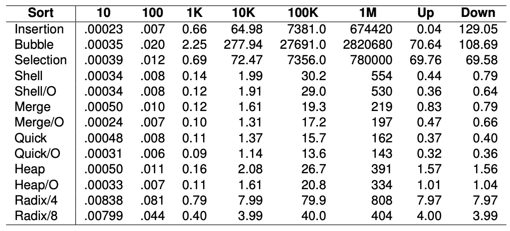
Growth speed : O(n)과 $O(n^2)$ 사이이다.
Exchange sorts(Insertion, Bubble, Selection)는 $O(n^2)$의 시간복잡도를 가지며 큰 인풋을 가질 때 가장 느리다.
Insertion sort는 거의 정렬되어 있을 때 가장 빠르다.
Quicksort와 mergesort가 가장 좋은 performance를 보인다.
radixsort는 k(# of digits) > $log_{r}n$일 때 O(n log n)보다 느리다.
radix/8은 radix/4보다 훨씬 빠르지만 많은 space를 사용한다.
또한 radix는 오로지 Integer 밖에 sort 가능하다.
10. Lower Bounds for Sorting
comparison-based sorting algorithms에서 가능한 lower bound를 구하고자 한다.
O(n log n)이 average, worst case에서 upper bound를 가지는 것을 알 수 있다.
I/O for sorting은 적어도 $\Omega(n)$이 걸린다.
우리는 Lower bound for sorting이 $\Omega(n log n)$이라는 것을 구할 예정

n개의 인풋에 대해 n!개의 permutation이 있을 수 있다.
sorting algorithm은 sorted list를 만들기 위한 결정을 하는 과정으로 볼 수 있다.
각각의 leaf node는 unique한 하나의 permutation을 의미한다.
comparison-based sorting algorithm은 무조건 n!개의 leaf node를 가진다.
n leaves를 가진 tree의 최소 높이는 얼마인가? $\Omega(logn)$
n! = $\sqrt{2\pi n}(\frac{n}{e})^n$ (Stirling's approximation)
$\Omega(log{n!})=\Omega(n log{n})$
lower bound가 $Omega(n log n)$이기 때문에 worst case에서 적어도 $Omega(n log n)$의 시간 복잡도를 가지게 된다.